Image compression - preliminaries
A monochromatic light source emits electromagnetic waves of one single frequency.
A typical human eye can detect waves with frequencies between around 400 and 790 terahertz.
Invisible ultra violet light and X-rays have higher frequencies, while infrared, microwaves and
radio frequencies are lower. Although lasers come close, monochromatic light does not really exist in
reality. Instead each light-source can be characterized by its
spectral density function.
If we wanted to capture a realistic color image of a given scene, we would have to store for
each pixel the spectrum of the light reaching it, i.e. a whole function of intensity vs. frequency.
Luckily our eyes are pretty lousy spectrometers and can be easily fooled. The retina of a typical human
eye contains four different kinds of photoreceptor cells, the three kinds of
cone cells (S,M and L types) being
responsible for our color perception. The three kinds differ in their sensitivity (or better: responsivity)
towards different frequencies. A given spectral density hitting a spot in they eye will create some
response like
S-cone: "I see almost nothing."
M-cone: "OMG! It's so bright!"
L-cone: "Meh, I give it a 6/10."
Which is translated by our brain to some color sensation: "I call it jonquil".
The interesting thing now is, that completely different spectral densities can lead to exactly the
same color sensation. In fact it is possible to fake a wide range of color sensations by
linearly combining three different light sources.
To make a long story short: to capture an image for human purposes, it is enough
to store for each pixel just the green, red and blue intensities that, when combined,
will lead to the same color sensation as the original spectrum. The 5-coned aliens
capturing our TV signals will find those artistic false color renderings amusing...
Loading images
MATLAB's powerful imread function can read several popular image formats (BMP, JPEG, PNG, CUR, PPM, GIF, PBM, RAS, HDF4, PCX, TIFF, ICO, PGM, XWD,...), many of which have several subclasses (grayscale, indexed, true-color, different bit-depths per channel, different compressions, etc...). We are interested in reading a non-compressed true-color TIFF image:
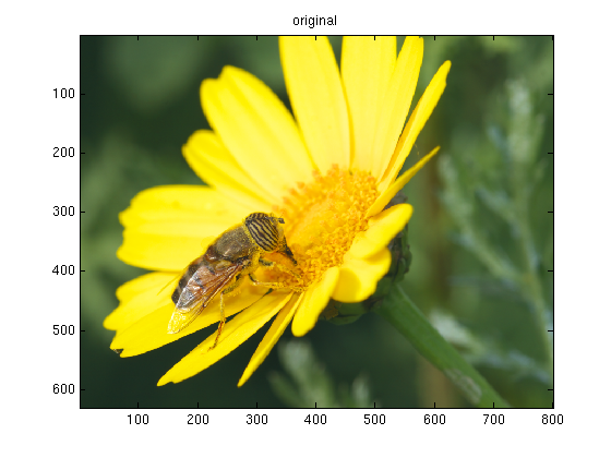
   % show_image.m
   % read and display a TIFF image
   dat = imread('test_image.tif');
   image(dat)
Feel free to use this test_image.tif if you have none of your own
at hand. This one was extracted from a camera raw file without invoking any compression that would
possibly reduce the information content of the file.
Let's see how MATLAB represents the image data:
   >> show_image
   >> whos dat
     Name        Size                 Bytes  Class    Attributes

     dat       630x800x3            1512000  uint8

   >> min(dat(:))

   ans =

       0

   >> max(dat(:))

   ans =

     255
The resolution of that image is 630 x 800 pixel. For each pixel there are 3 integer values between 0
and 255 stored. These correspond to the red, green and blue intensities of each pixel. One byte (8 bit)
are needed to store each color entry, so we have a total of 24 bits per pixel. This is a standard
bit-depth in the computer world. Raw files of modern cameras usually have a higher color
depth which is why exposure corrections
are possible to some degree in post-processing.
All this information and much more can be obtained with the command
imfinfo.
E.g. in our example
imi = imfinfo('test_image.tif')
Manipulating images
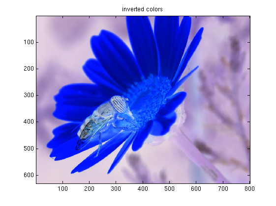
We can modify the dat matrix before drawing it. The possibilities are endless. Here some simple examples
- Invert colors, or make a negative image. For each pixel we map [r,g,b] -> [255-r, 255-g, 255-b], where r,g and b are the red, green and blue intensities of that pixel.
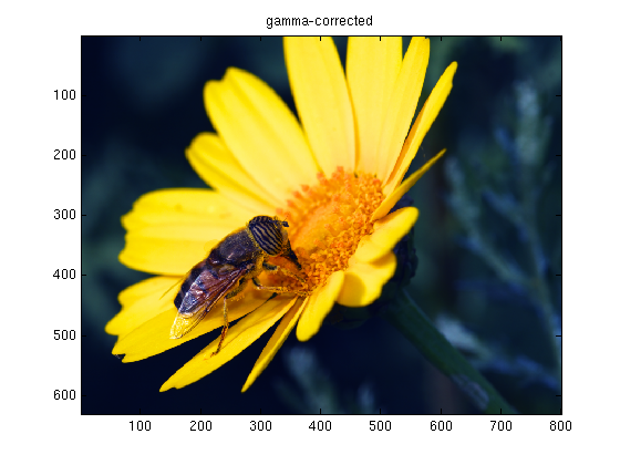
- Change the gamma. We map the intensities onto an interval 0...1, and apply the mapping r -> r^gamma. In the end they are mapped back onto integers 0...255. We can assign different gammas to each color channel. Of course other maps in place of the power function are possible and will lead to possibly interesting results (the functions should be strictly non-negative).
- Blur filter. For each color channel the pixel at coordinates (x,y) is
replaced by the weighted average
of itself (weight 1) with its four nearest neighbors (weight alpha). E.g. for the red channel
r(x,y) <- [r(x,y) + alpha * (r(x+1,y) + r(x-1,y) + r(x,y+1) + r(x,y-1))] / (1+4*alpha)
This is repeated N times for all pixels. To avoid complications with boundary pixels the example smears only the center of the image. - ...
here a possible implementation
   % manipulate.m
   % read and manipulate images
   dat = imread('test_image.tif');

   figure()
   image(dat)
   title('original')

   % invert colors
   dat2 = 255-dat;
   figure();
   image(dat2);
   title('inverted colors');

   % gamma-correction
   gamma_r = 2.2;  % gamma correction red channel
   gamma_g = 2.0;  % gamma correction green channel
   gamma_b = 1.0;  % gamma correction blue channel

   dat2(:,:,1) = uint8( (double(dat(:,:,1))/256).^gamma_r *256);
   dat2(:,:,2) = uint8( (double(dat(:,:,2))/256).^gamma_g *256);
   dat2(:,:,3) = uint8( (double(dat(:,:,3))/256).^gamma_b *256);
   figure();
   image(dat2);
   title('gamma-corrected');

   % blur filter for central 301x301 pixels
   alpha =0.8;
   N = 30;
   dat2 = double(dat);
   [height,width] = size(dat(:,:,1));
   cx = round(width/2);
   cy = round(height/2);
   for n=1:N
      tmp = 1/(1+4*alpha) * (        dat2(cy-150:cy+150,cx-150:cx+150,:) + ...
                              alpha*(dat2(cy-150-1:cy+150-1,cx-150:cx+150,:)+ ...
                                     dat2(cy-150+1:cy+150+1,cx-150:cx+150,:)+ ...
                                     dat2(cy-150:cy+150,cx-150-1:cx+150-1,:)+ ...
                                     dat2(cy-150:cy+150,cx-150+1:cx+150+1,:)));
      dat2(cy-150:cy+150,cx-150:cx+150,:) = tmp;
   end
   dat2 = uint8(dat2);
   figure();
   image(dat2);
   title('blurred');
The output should resemble:

Homework: pick your favorite filter from gimp or photoshop and try to reproduce it in MATLAB. You can store the final results using imwrite. Enjoy!
Everything from here on will be about manipulating the image data such that the required storage
is reduced while the perceived image remains almost the same.
The next part is about
down-sampling and interpolating.