Image compression - downsampling and interpolating
In the previous section we've seen how to load true-color images,
how MATLAB represents the image data as a matrix for each color, and how these matrices can be
fooled around with.
In this part the possibly simplest method of image compression is
introduced.
Downsampling
The test image has a resolution of 630 x 800 pixel. Which at 24 bit/pixel
makes roughly 1.5 MB. A crude compression method would be to throw away 3/4 of the information by averaging
four neighboring pixels and storing only one color triplet for each four pixels
For a 16 x 16 cutout (tip of the antenna of the hooverfly) of the test image this will look like (here's
the code for the figs):
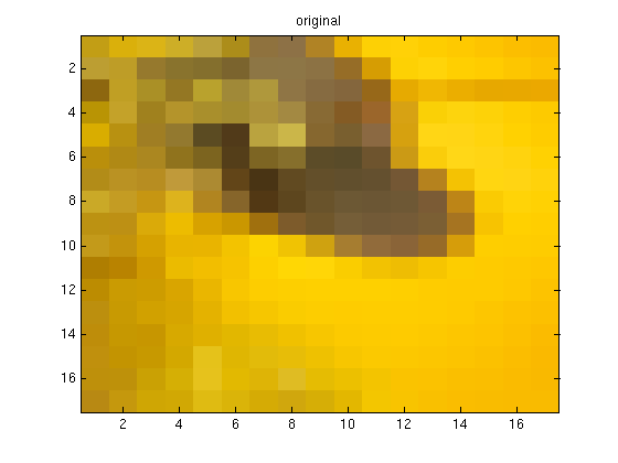
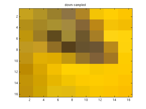
The storage space is reduced to 1/4 of the original. So is the information content and with it
the image quality.
Interpolating
3/4 of the information are gone and cannot be recovered. But can we
maybe soothe the consequences a bit? If we look at one color channel
and in one direction only, what we have done is (blocks are 4 pixels now):
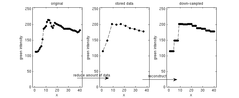
The "reconstruct" step employed here is only one (the simplest) way of filling
the gaps. What we have done is called a piecewise constant interpolation. There
are more refined ways of interpolating.
Interpolation is a common task and MATLAB provides user-friendly built-in functions:
interp1 (interpolation in 1D) and
interp2 (interpolation in 2D).
For instance linear and spline interpolations in 1D would look like this (code):
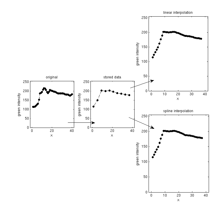
The final results of those two in this case are very similar. They look much smoother than
the piecewise constant interpolation, but not necessarily closer to the original data.
The smoother the original data, the better interpolation will work.
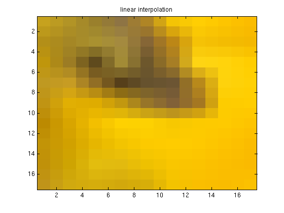
Let's go back to our first two dimensional example. The following code
performs linear and spline interpolations after reducing the data by a factor of
1/2 x 1/2.
   % downsample4.m

   dat = imread('test_image.tif');
   dat2 = dat(310:327,334:351,:);
   clear dat;

   [h,w,dummy] = size(dat2);
   dat2 = double(dat2);

   % reduce the data. Average 2x2 blocks
   for lx=1:w/2,
   for ly=1:h/2,
      x = (lx-1)*2+1;
      y = (ly-1)*2+1;
      dat_reduced(ly,lx,1) = (dat2(y,x,1) + dat2(y+1,x,1) + dat2(y,x+1,1) + dat2(y+1,x+1,1))/4;
      dat_reduced(ly,lx,2) = (dat2(y,x,2) + dat2(y+1,x,2) + dat2(y,x+1,2) + dat2(y+1,x+1,2))/4;
      dat_reduced(ly,lx,3) = (dat2(y,x,3) + dat2(y+1,x,3) + dat2(y,x+1,3) + dat2(y+1,x+1,3))/4;
   end
   end

   % use interpolation methods to reconstruct an image
   % of the original size

   dat_reconstructed = zeros(h-1,w-1,3);

   dat_reconstructed(:,:,1) = interp2([1:2:h],[1:2:w]',dat_reduced(:,:,1), [1:h-1],[1:w-1]','linear');
   dat_reconstructed(:,:,2) = interp2([1:2:h],[1:2:w]',dat_reduced(:,:,2), [1:h-1],[1:w-1]','linear');
   dat_reconstructed(:,:,3) = interp2([1:2:h],[1:2:w]',dat_reduced(:,:,3), [1:h-1],[1:w-1]','linear');
   dat_reconstructed = uint8(dat_reconstructed);
   figure();
   image(dat_reconstructed);
   title('linear interpolation');

   dat_reconstructed(:,:,1) = interp2([1:2:h],[1:2:w]',dat_reduced(:,:,1), [1:h-1],[1:w-1]','spline');
   dat_reconstructed(:,:,2) = interp2([1:2:h],[1:2:w]',dat_reduced(:,:,2), [1:h-1],[1:w-1]','spline');
   dat_reconstructed(:,:,3) = interp2([1:2:h],[1:2:w]',dat_reduced(:,:,3), [1:h-1],[1:w-1]','spline');
   dat_reconstructed = uint8(dat_reconstructed);
   figure();
   image(dat_reconstructed);
   title('spline interpolation');
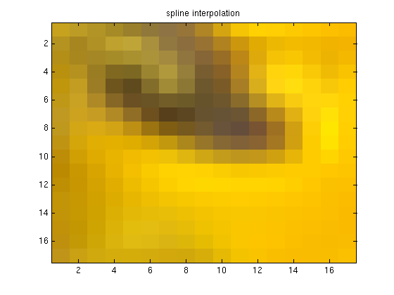
Notice how the spline interpolation creates funny artifacts (bright yellow halo around the dark area).
Two remarks to the code:
- We reconstruct an image that is smaller by 1 pixel in each direction than the original image. That's because interpolation needs pixels on both sides to work.
- In the interp2 command x has to be a row and y a column vector.
Selective downsampling
Downsampling works well where the original image is smooth. Often images have large smooth areas
(skies, out-of-focus areas). An idea would be to use downsampling only for these parts of the image.
This would require a clever partitioning algorithm. In this tutorial we will pursue a different
direction.
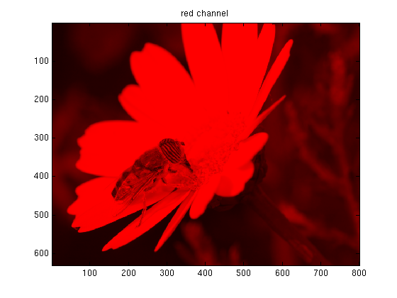
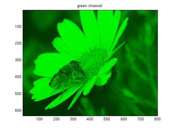
We have three different color channels that we treated equally so far. The dominant colors
in our test-picture are green and yellow (which is a mixture of red and green).
So we don't expect the blue channel to be particularly important for this particular picture and can try
to down-sample only the blue channel. In the example below we choose rather large 8x8 blocks. The
final result is written out into a file so that original and
reconstructed images can be compared in full resolution.
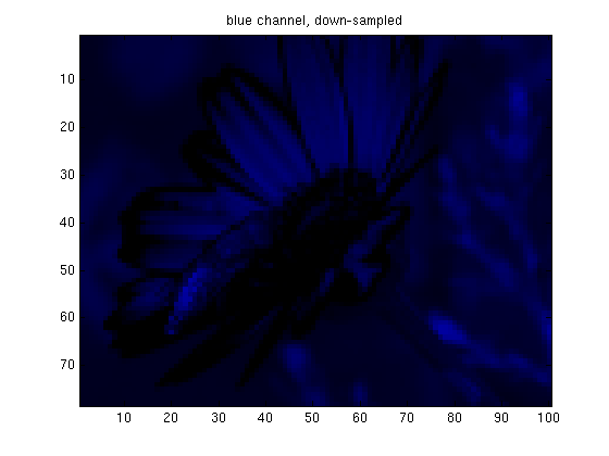
   % compress1.m
   dat = imread('test_image.tif');


   % reduce resolution of blue layer by factor 64 (block 8x8 pixels)

   [height,width] = size(dat(:,:,1));

   % down-sampling
   for w=1:width/8,
   for h=1:height/8,
      blue(h,w) = mean(mean(dat((h-1)*8+1:h*8,(w-1)*8+1:w*8, 3)));
   end
   end

   image(dat); title('original');

   figure()
   image(dat(:,:,1)); title('red channel');
   c = zeros(256,3);            % setup a color axis with red intensities
   c(:,1) = 0:1/255:1;
   colormap(c); caxis([0 255]);

   figure()
   image(dat(:,:,2)); title('green channel');
   c = zeros(256,3);            % setup a color axis with green intensities
   c(:,2) = 0:1/255:1;
   colormap(c); caxis([0 255]);

   figure()
   image(dat(:,:,3)); title('blue channel');
   c = zeros(256,3);            % setup a color axis with blue intensities
   c(:,3) = 0:1/255:1;
   colormap(c); caxis([0 255]);


   figure();
   image(blue); title('blue channel, down-sampled');
   c = zeros(256,3);
   c(:,3) = 0:1/255:1;
   colormap(c); caxis([0 255]);


   % reconstruct a complete image from reduced blue data
   % interpolate linearly

   [hes,wis] = size(blue);
   dat(:,:,3) = interp2([1:width/wis:width],[1:height/hes:height]',blue,[1:width],[1:height]','linear');
   figure();
   image(dat); title('reconstructed image (linear interpolation)');

   imwrite(dat,'test_image_blue64.tif','TIFF');
Among others, the script draws the three color channels separately
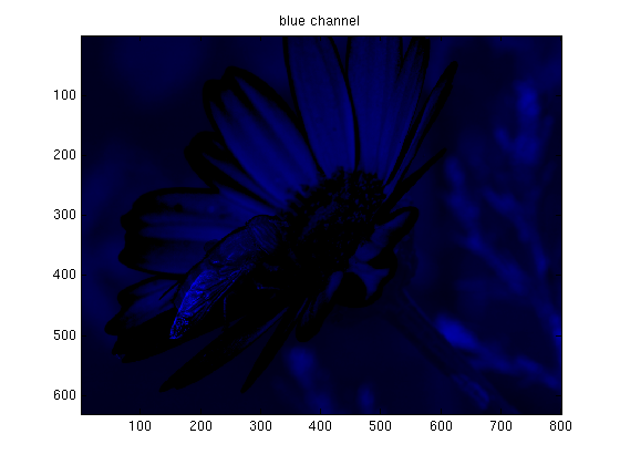
And the down-sampled blue channel (Note that the
true resolution of the images is higher than plotted.
Nevertheless the large 8x8 blocks are clearly visible).
Overall the compressed image needs 67% of the space of the original one and the image quality of the result is not too bad. Some compression artifacts are visible on the wing of the fly. The idea of down-sampling only "unimportant" channels works, but
- How to decide which channels are important?
- What if all channels are equally crucial for a detailed reproduction?
The next part of the tutorial addresses both questions. The strategy is to "rotate" the image into a different color space, in which it is more clear which channels are important.