Image compression - Fourier transforms
We've seen how to apply coordinate transformations to change to a more suitable color space. In this section we'll get to know another family of linear transformations that are extremely useful, not only for compression of data, but in many fields of mathematics, physics and engineering. There's tons of material on the subject online (you could start for instance from here), so I will try to keep things short. In particular I'll focus exclusively on the discreet Fourier transform (DFT) and its relatives.
DFT
Given a vector f with N components we have seen that an invertible N x N matrix can be used to change to a different coordinate system.
In the new system the coordinates are given by
F = A*f
To get back one uses the inverse map
f = inv(A)*F
The transformation known as discrete Fourier transform has a matrix A with the k'th row and j'th column given by
A(k,j) = exp( -2i * π * (k-1) * (j-1) / N)
There are various other conventions on the market, but this is the one that is also used by MATLAB's built in functions.
A typical vector to apply the transformation to could be for instance one row of one channel of an image. The components
of the transformed vector F can be interpreted as frequencies. Often the frequency spectrum is concentrated around 0 and
one can discard high frequencies in order to save storage space. This is demonstrated in the following example
   % dft1.m

   dat = imread('test_image.tif');
   f = double(dat(50,:,1)).'; % example data: 50th row of red channel

   N=length(dat);
   for k=1:N,
   for j=1:N,
      A(k,j) = exp(-2i*pi*(k-1)*(j-1)/N);
   end
   end

   F = A*f;

   subplot(3,1,1);
   plot(f,'k-'); xlabel('j'); ylabel('Intensity'); title('original data');
   subplot(3,1,2);
   plot(real(F),'k-'); axis([0 800 -1e4 1e4]); hold on;
   plot(imag(F),'r-'); xlabel('k'); ylabel('F'); title('Fourier transformed data');


   max(inv(A)*F - f) % indeed, it is the inverse...
   max(F - fft(f))   % indeed, the conventions equal MATLAB's

   F(100:700)=0;     % Throw away high frequency information
   subplot(3,1,3);
   fnew = real(inv(A)*F);
   plot(fnew,'k-'); xlabel('j'); ylabel('Intensity'); title('reconstructed from 200 low frequency modes');
The output:
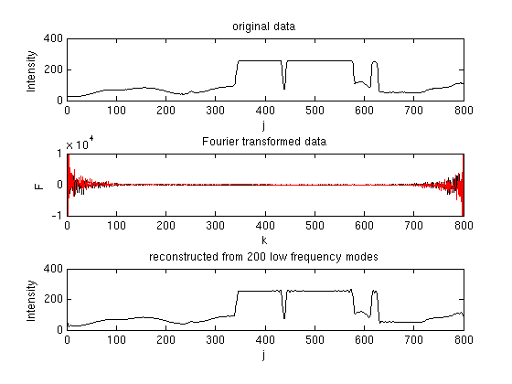
OK, the DFT and its inverse clearly work and agree with MATLAB's. Most of the frequency spectrum is contained between k=1..100
(values 700..800 are known due to symmetries, discussed in a sek). Throwing away the higher frequencies before performing the inverse transform,
results in a good approximation to the original data. Typical artifacts are visible in constant areas and whenever
high slopes or sharp edges occur.
Some further remarks are in order
- The Fourier transoform is complex, so, for real input the data has apparently doubled.
However it looks symmetric. That's because for real vectors f the relation
conj(F(k)) = F(N-k+2)
holds (for components k=2...N/2). The k=1 component is real, so altogether there are only N independent components in the transformed vector. - A matrix-vector multiplication takes ∝N^2 operations. A clever algorithm, called fast Fourier transform, or FFT, performs this particular matrix-vector multiplication in ∝N log(N) operations. MATLAB/octave provide the built-in functions fft and the inverse ifft.
- To perform a two dimensional Fourier transform, one can first transform all rows, and then all columns. The total number of operations is ∝ 2*N^3 or, using fast Fourier transform (fft2, ifft2) ∝ 2*N^2*log(N).
- The original data was an 8 bit integer per component. Now we have a 128 bit complex number per component. Can this be reduced?
- Is there a more subtle possibility of compression than simply cutting away the high frequencies?
The answer the last two points is "yes". A transformation related to the DFT will help us getting rid of the imaginary parts, and a possible compression that does not simply cut away high frequencies consists in dividing a given frequency by some constant and rounding to the next integer. Details will follow.
Discrete cosine transform
A transformation particularly suited for real inputs is the cosine transform. The transformed vector
F remains real. The transformation matrix is given by
A(k,j) = w(k) * cos( π * (k-1) * (j-1/2) / N)
with w(1) = sqrt(1/N) and w(2..N) = sqrt(2/N).
In practice the matrix does not need to be constructed, but it is
necessary to know the inverse
A-1(k,j)= w(j) * cos( π * (j-1) * (k-1/2) / N).
MATLAB provides two dimensional discrete cosine transforms with
its image processing toolbox
(dct2,
idct2).
The implementation uses FFT algorithms and a relation between DFTs and cosine transforms
to carry out the transformation. For readers without the toolbox, and for pedagogical reasons,
here a much slower, but simpler implementation:
   % dct2.m
   % discrete cosine transform in 2d
   % (painfully slow)

   function F = dct2(f)

   [m,n] = size(f);
   F = zeros(m,n);

   % transform rows
   k=(2*[1:n]-1)*pi/n/2;
   w=[sqrt(0.5); ones(n-1,1)]*sqrt(2/n);
   for ml=1:m
      for nl=1:n
         F(ml,nl) = w(nl) * sum( f(ml,:) .* cos(k.*(nl-1)) );
      end
   end

   % transform columns
   f=F;
   k=(2*[1:m]'-1)*pi/m/2;
   w=[sqrt(0.5); ones(m-1,1)]*sqrt(2/m);
   for nl=1:n
      for ml=1:m
         F(ml,nl) = w(ml) * sum( f(:,nl) .* cos(k.*(ml-1)) );
      end
   end
The code for the inverse transform is almost identical: idct2.m. A quick test confirms that it really is the inverse (to machine precision):
   >> dat = rand(5,7);
   >> max(max(idct2(dct2(dat))-dat))

   ans =

      3.3307e-16
Quantization
The cosine transform leaves us with an array of double precision numbers. When these are rounded to
the next integer in order to save some space, some information is lost. One can go further and divide the number
by some integer before rounding. This is called quantization. For instance, if the quantization number is 16 and the
data point 1234.56, we would have to store:
round(1234.56/16) = 77
To recover the original value we just multiply by the quantization number
77 * 16 = 1232
Obviously some detail is lost. The bigger the quantization number, the further from the original we can
end up. It turns out that in typical images it is more difficult to spot the resulting artifacts
for high frequencies than for low ones. A natural consequence is to use a quantization matrix Q, and round the
cosine transformed image F according to
W = round(W./Q)
The entries in Q corresponding to small frequencies (upper left corner) would have to be smaller
than the ones corresponding to large ones. The last problem: Q is as large as the original image,
so the data has doubled. JPEG's solution is to divide the original image into blocks of size 8x8
and treat all of them separately. Each block is cosine transformed and subsequently quantized.
Only one quantization matrix of size 8x8 is needed in the whole procedure. How the method works,
and what the typical artifacts are is demonstrated in the following code:
% dct_demo.m

   dat = imread('test_image.tif');
   [m,n] = size(dat(:,:,1));
   m = floor(m/8)*8; % to make things easier: make dimensions multiples of 8
   n = floor(n/8)*8;

   r = dat(1:m,1:n,1);
   g = dat(1:m,1:n,2);
   b = dat(1:m,1:n,3);
   Y  = uint8(      0.299   *r +  0.587   *g  +  0.114   *b);

   figure();
   imagesc(Y); title('original'); colormap(gray);
   imwrite(Y,'original_bw.tif','TIFF','Compression','none');

   % quantization matrix
   Q = [16  11  10  16  24  40  51  61; ...
        12  12  14  19  26  58  60  55; ...
        14  13  16  24  40  57  69  56; ...
        14  17  22  29  51  87  80  62; ...
        18  22  37  56  68 109 103  77; ...
        24  35  55  64  81 104 113  92; ...
        49  64  78  87 103 121 120 101; ...
        72  92  95  98 112 100 103  99];

   Ytransformed = zeros(m,n);

   % loop over 8x8 blocks
   for bx = 1:m/8
   for by = 1:n/8
      block = double(Y(bx*8-7:bx*8, by*8-7:by*8))-128; % get block, and shift it
      block = dct2(block);                             % discrete cosine transform
      block = round(block ./ Q);                       % quantization
      Ytransformed(bx*8-7:bx*8, by*8-7:by*8) = block;
   end
   end


   clear r g b Y
   Y = uint8(zeros(m,n));

   % reconstruct Y channel
   for bx = 1:m/8
   for by = 1:n/8
      block = Ytransformed(bx*8-7:bx*8, by*8-7:by*8); % get block
      block = block.*Q;                               % dequantization
      block = idct2(block);                           % inverse discrete cosine transform
      block = uint8(block + 128);                     % shift
      Y(bx*8-7:bx*8, by*8-7:by*8) = block;
   end
   end

   figure();
   imagesc(Y); title('reconstructed'); colormap(gray);
   imwrite(Y,'reconstructed_bw.tif','TIFF','Compression','none');
For simplicity the code works just on the luma channel of our test image where γ=1 was (wrongly) assumed.
The image is subdivided into blocks of 8 x 8 pixels. Each block is cosine-transformed and quantized.
The process is then inverted and the original image (original_bw.tif) as well as
the reconstructed one (reconstructed_bw.tif) are saved for later
comparison.
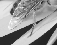
The quantization is the main cause of compression artifacts. If we compare crops from the original (upper) and
the reconstructed (lower) image carefully, we quickly find artifacts that are typical for the JPEG compression.

So far we've seen what we have lost, but where is the gain? The original matrix (Y in the code) has the same size as
the transformed and quantized one (Ytransformed), so where is the compression?
- The compression is just about to happen! If we count the occurrences of different integers in Ytransformed,
we see that 93.7% of the entries are zeros. Another 1.3% are ones and only the remaining few have higher values.
A very popular lossless compression algorithm takes advantage of this imbalance. It is described in some detail
in the following section on Huffman coding, which is also the last technical part
of this JPEG compression tutorial.